团团虾声明:本文翻译自 vLLM 官方博客 Next-Level Inference: Why Your Single-Node vLLM Setup Needs Prefill-Decode Disaggregation,作者 AMD and Embedded LLM。原文发表于 2026 年 4 月 7 日。
TL;DR: Prefill 和 decode 在同一个 GPU 上相互竞争,在高负载下导致 ITL(Token 间延迟)尖峰。本文展示如何在一台 8-GPU MI300X 节点上,使用 AMD 的 MORI-IO connector 实现 PD 分离——相比同一 8 块 GPU 上的标准混杂部署,goodput 提升 2.5 倍,同时实现稳定的 token 生成。基准测试使用 Qwen3-235B-A22B-FP8 模型,8 req/s,2000 token 输入,1000 token 输出——完整配置见表 3 和”实验细节”章节。
引言
在之前关于 MoE 优化的探索中 [1],我们介绍了如何在一台 8-GPU AMD Instinct MI300X 节点上,通过 Tensor、Pipeline、Data 和 Expert Parallelism 分布式部署大型模型。本文展示 Prefill-Decode 分离——由 AMD 的 MORI-IO 驱动——如何解决这一瓶颈,在不需要多节点集群的情况下,提供更高的 goodput 和更可预测的性能。
你的 HBM 已充分利用、计算已良好均衡、vLLM 部署运行平稳——直到你提高并发度。然后事情开始恶化:ITL(Inter-Token Latency,Token 间延迟)不可预测地飙升。根因很简单——prefill 和 decode 本质上是不同的工作负载,却在竞争同一 GPU 资源。
Prefill 是计算密集型的: 它通过大规模的 GEMM 操作并行处理整个 prompt,成本随输入长度线性增长。
Decode 是内存带宽密集型的: 它逐 token 生成,反复从 HBM 加载模型权重,每字节的计算量相对较低。
当两个阶段共享同一个实例时,它们会相互干扰。Prefill 请求可能阻塞几十个正在进行的 decode 流,导致明显的卡顿;同时 decode 工作负载会延迟新 prefill 的调度。结果是两个阶段都无法高效或可预测地运行。
关键亮点
- 在相同硬件上实现 2.5 倍 Goodput。 通过分离 prefill 和 decode,在同一台 8-GPU MI300X 节点上实现显著更高的 SLO 合规吞吐。
- 消除负载下的 ITL 尖峰。 专用 decode GPU 通过移除 prefill 干扰,确保稳定、可预测的 token 生成。
- 单节点分离——无需集群。 完全在一个节点内实现 Prefill-Decode(PD)分离,释放未利用的性能。
- MORI-IO 实现快速 KV cache 传输。 基于 RDMA 的 KV 搬运实现了阶段间的高效交接。
- 灵活的模式与权衡。 Write 模式提供最佳性能(更低的 TTFT),而 Read 模式提供更简单的编排——两者都远远优于标准部署。
常见误解:“分离只有数据中心集群才需要”
当推理工程师听到”Prefill-Decode(PD)分离”时,他们通常会想到多节点数据中心部署——专用 prefill 节点、专用 decode 节点,以及将它们连接在一起的 RDMA 网络。自然的假设是:“我只有一个 8-GPU 节点——这不适用于我。”
这个假设浪费了大量的性能。PD 分离完全可以在一台 8-GPU 系统内实现,如果你需要满足严格的延迟 SLO,这往往才是正确的做法。
思路很直接:将两个阶段分离到专用实例。例如,四块 GPU 处理 prefill,另外四块处理 decode。每个实例可以独立地确定规模、并行度和调度方式,消除了限制整体式部署的头端阻塞(head-of-line blocking)。
挑战在于交接。Prefill 阶段产生的 KV cache 必须传输到 decode 实例——这涉及 GB 级别的数据。如果处理不当,传输本身可能成为新的瓶颈,抵消分离的好处。
AMD 通过 MORI-IO 解决了这个问题。MORI-IO 是一个基于 RDMA 的 KV cache connector,已贡献给 vLLM [4],构建在开源 MORI(Modular RDMA Interface)[5] 框架之上。
范围: 本文聚焦于单节点 PD 分离,部署在一台 8-GPU 的机器上,旨在提升你现有硬件上的 goodput。
架构:基于 PD 分离的推理服务
将你的节点拆分,需要从整体式部署转向轻量级微服务架构,包含三个组件,如下表 1 所示:
| 组件 | 角色 |
|---|---|
| Prefill 实例 | 处理输入 prompt,产生 KV cache(GPU 0–3) |
| Decode 实例 | 使用传输过来的 KV cache 逐 token 生成输出(GPU 4–7) |
| Proxy 服务器 | 客户端请求入口;首先路由到 prefill,然后到 decode |
高层次上看,两种模式都将 KV cache(prefill 的输出)从 prefill 实例传输到 decode 实例,但区别在于谁发起传输以及何时传输:
- Read 模式: Proxy 等待 prefill 完成,然后将 KV block 位置转发给 decode。Decode 在开始生成前通过 RDMA 拉取 KV 数据。
- Write 模式: Proxy 同时向 prefill 和 decode 分派请求。Prefill 在计算每一层时,直接将 KV 数据推入 decode 的内存——因此 prefill 一完成,decode 就可以开始生成。
请求流程详解
MORI-IO 支持两种传输模式,区别在于谁发起 RDMA 传输以及 proxy 如何编排两个阶段。通过环境变量 VLLM_MORIIO_CONNECTOR_READ_MODE 设置。
Read 模式——Decode 拉取 KV cache
启用方式:export VLLM_MORIIO_CONNECTOR_READ_MODE=1
在 read 模式下,proxy 按顺序分派给 prefill 和 decode:它等待 prefill 完成,提取远端 block ID,然后将它们转发给 decode。Decode 实例使用这些 ID 通过 RDMA 从 prefill 拉取 KV cache。请求流程如图 1 所示。

单次请求的时间顺序序列:
- Client → Proxy: 客户端发送推理请求。
- Proxy → Prefill: Proxy 将 prompt 路由到 prefill 实例(
max_tokens=1)。 - Prefill → Proxy(响应): Prefill 返回
remote_block_ids和remote_engine_id,标识 KV cache 所在位置。 - Proxy → Decode: Proxy 将请求(含远端 block ID)转发给 decode。
- Decode 拉取 KV cache(WAITING_FOR_REMOTE_KVS): Decode 对 prefill 的内存发起 RDMA 读取。调度器在传输完成前跳过该请求。
- Decode → Prefill(清理): 所有 KV block 传输完成后,decode 通知 prefill 释放其 block。
- Decode → Proxy → Client: 生成的 token 通过 SSE 流式返回。
Write 模式——Prefill 推送 KV cache(默认)
启用方式:不设置 VLLM_MORIIO_CONNECTOR_READ_MODE(或设为 0)
在 write 模式下,proxy 并发地向 prefill 和 decode 分派——不等 prefill 先完成。Prefill 实例在逐层计算的同时,将 KV cache 逐层直接推送到 decode 实例预分配的内存中。请求流程如图 2 所示。

单次请求的时间顺序序列:
- Client → Proxy: 客户端发送推理请求。
- Proxy → Prefill 和 Proxy → Decode(并发): Proxy 并行触发两个请求。Prefill 请求携带 decode 的连接信息;decode 请求携带 prefill 的连接信息。Proxy 不阻塞等待 prefill 响应。
- Prefill 推送 KV cache: 每计算完一层,
save_kv_layer发起 RDMA write,直接写入 decode 实例预分配的 KV block 内存。在 chunked prefill 中,block 累积到最后一个 chunk 时发起写入。 - Decode 等待写入完成(WAITING_FOR_REMOTE_KVS): Decode 调度器每一步轮询
pop_finished_write_req_ids,直到所有 block 到达。 - Decode 生成: 一旦所有 KV block 到达,decode 立即将请求移到 ready 队列,开始自回归生成。
- Decode → Proxy → Client: 生成的 token 通过 SSE 流式返回。
Proxy 中的关键代码差异是一个简单的条件分支:
# examples/online_serving/disaggregated_serving/moriio_toy_proxy_server.py

if TRANSFER_TYPE == "READ":
    # 串行:等待 prefill 完成,提取 block ID 供 decode 拉取
    prefill_response = await send_prefill_task
    req_data["kv_transfer_params"]["remote_engine_id"] = prefill_response[
        "kv_transfer_params"
    ]["remote_engine_id"]
    req_data["kv_transfer_params"]["remote_block_ids"] = prefill_response[
        "kv_transfer_params"
    ]["remote_block_ids"]

# 在 WRITE 模式下,此处立即向下执行——
# 不会 await send_prefill_task。两个阶段已在飞行中。
decode_request_task = asyncio.create_task(
    start_decode_request(decode_instance_endpoint["request_address"], req_data, request_id)
)
在 read 模式下,remote_block_ids 必须通过 proxy 中转,因为 decode 需要知道要从 prefill 侧拉取哪些具体的 block。在 write 模式下,prefill 拥有写入权,直接将数据推送到 decode 的地址——不需要中转 block ID。
Read 模式 vs Write 模式:一目了然
底层上,MORI-IO(在 vLLM 中作为 MoRIIOConnector 暴露)管理 KV cache 的交接。无论何种传输模式,在实例对之间首次 RDMA 传输之前,MORI-IO 会通过 ZMQ 进行一次性的元数据交换——共享 KV cache 基地址、block 大小和每层 tensor 步长。这一步握手在后台线程中异步运行,不阻塞引擎循环,产生的 RDMA 会话缓存后用于所有后续请求。
两种模式共享相同的握手和 RDMA 传输机制——区别完全在于 proxy 的分派层和传输方向。表 2 一目了然地展示了关键区别:
| 属性 | Read 模式 | Write 模式 |
|---|---|---|
VLLM_MORIIO_CONNECTOR_READ_MODE | =1 | 不设置(或 =0) |
| RDMA 方向 | Decode 从 prefill 拉取 | Prefill 推送到 decode |
| Proxy 分派 | 串行(await prefill → 分派 decode) | 并发(prefill 和 decode 并行) |
通过 proxy 中转 remote_block_ids | 需要 | 不需要 |
| KV 清理信号 | Decode 在拉取后通知 prefill 释放 block | Prefill 按请求跟踪写入完成 |
结果:2.5 倍 Goodput
深入具体配置之前,先看看分离实际能带来什么。
为什么用 Goodput,而不是 Throughput
单纯的吞吐量具有误导性——一个系统可能在维持高请求率的同时,默默违反大多数用户的延迟目标。我们使用 goodput 作为主要指标,遵循 DistServe 方法论 [3]:
Goodput = 最大请求率(req/s),使得请求同时满足 TTFT < T_ttft 和 ITL < T_itl。
这在一个数字中同时捕获了成本(每秒请求数)和服务质量(延迟 SLO 达成率)。我们的 SLO 目标:TTFT < 1 秒且 ITL < 50 毫秒/每 token。一个请求只有两个条件都满足才算入 goodput。
核心结果
图 3 展示了请求率 = 8 时的 goodput:
| 指标 | Standard (1× TP8) | Standard (2× TP4) | MORI-IO Read (1P+1D) | MORI-IO Write (1P+1D) |
|---|---|---|---|---|
| 满足两个 SLO 的请求 | 26/100 | 30/100 | 70/100 | 73/100 |
| 主要失败模式 | ITL 尖峰(P99 ITL >> 50 ms) | ITL 尖峰(双峰:~30ms 和 ~150ms) | 部分请求 TTFT 超过 1s | 部分请求 TTFT 超过 1s |
| 相对 goodput | 0.9x | 1x | 2.4x | 2.5x |
标准部署失败的原因是 ITL 集中在两个聚类——高延迟聚类 ~150ms 远超 50ms 阈值。两种分离模式完全消除了 ITL 违规;它们余下的失败是随着请求率上升的 TTFT 超标。Write 模式微弱领先于 read 模式(73 vs 70),因为并发 proxy 分派降低了 TTFT,使更多请求保持在 1s 阈值以下。
groups.forEach(function(g) {
  var n = g.x.length;
  var ttftColors = [];
  var itlColors = [];
  for (var i = 0; i < n; i++) {
    var failed = (g.ttft[i] >= ttftThreshold) || (g.itl[i] >= itlThreshold);
    ttftColors.push(failed ? grayColor : g.color);
    itlColors.push(failed ? grayColor : g.color);
  }
  // TTFT trace (top)
  traces.push({
    name: g.name,
    type: 'bar',
    x: g.x,
    y: g.ttft,
    marker: {color: ttftColors, line: {width: 0.5, color: 'rgba(0,0,0,0.4)'}},
    legendgroup: g.name,
    showlegend: false,
    xaxis: 'x', yaxis: 'y',
    hovertemplate: '<b>' + g.name + '</b> req #%{x}<br>TTFT: %{y:.4f} s<extra></extra>'
  });
  // ITL trace (bottom)
  traces.push({
    name: g.name,
    type: 'bar',
    x: g.x,
    y: g.itl,
    marker: {color: itlColors, line: {width: 0.5, color: 'rgba(0,0,0,0.4)'}},
    legendgroup: g.name,
    showlegend: false,
    xaxis: 'x', yaxis: 'y2',
    hovertemplate: '<b>' + g.name + '</b> req #%{x}<br>ITL: %{y:.4f} s<extra></extra>'
  });
});
return traces;
}
var layout = { title: {text: ‘TTFT per request (top) / ITL per request (bottom)’}, grid: {rows: 2, columns: 1, pattern: ‘independent’}, barmode: ‘overlay’, bargap: 0, legend: {x: 0.5, y: -0.08, orientation: ‘h’}, xaxis: {range: [-0.5, 399.5]}, yaxis: {title: ‘TTFT (s)’, range: [0, 1.75]}, yaxis2: {title: ‘ITL (s)’, range: [0.22, 0]}, shapes: [ {type: ‘rect’, x0: -0.5, x1: 99.5, y0: 0, y1: 1.75, fillcolor: ‘#eef’, layer: ‘below’, opacity: 0.15, line: {width: 0}}, {type: ‘rect’, x0: 99.5, x1: 199.5, y0: 0, y1: 1.75, fillcolor: ‘#efe’, layer: ‘below’, opacity: 0.1, line: {width: 0}}, {type: ‘rect’, x0: 199.5, x1: 299.5, y0: 0, y1: 1.75, fillcolor: ‘#fee’, layer: ‘below’, opacity: 0.1, line: {width: 0}}, {type: ‘rect’, x0: 299.5, x1: 399.5, y0: 0, y1: 1.75, fillcolor: ‘#ffe’, layer: ‘below’, opacity: 0.1, line: {width: 0}}, ], annotations: [ {x: 49.5, y: 1.68, text: ‘Standard (1× TP8)’, showarrow: false, font: {size: 11, color: ‘#9467bd’}, xanchor: ‘center’}, {x: 149.5, y: 1.68, text: ‘Standard (2× TP4)’, showarrow: false, font: {size: 11, color: ‘#1f77b4’}, xanchor: ‘center’}, {x: 249.5, y: 1.68, text: ‘MORI-IO Read (1P+1D)’, showarrow: false, font: {size: 11, color: ‘#ff7f0e’}, xanchor: ‘center’}, {x: 349.5, y: 1.68, text: ‘MORI-IO Write (1P+1D)’, showarrow: false, font: {size: 11, color: ‘#2ca02c’}, xanchor: ‘center’}, ], hovermode: ‘closest’, margin: {l: 60, r: 20, t: 40, b: 80} };
function updateChart() { var ttftVal = parseFloat(document.getElementById(‘fig3-ttft-slider’).value); var itlVal = parseFloat(document.getElementById(‘fig3-itl-slider’).value); document.getElementById(‘fig3-ttft-label’).textContent = ttftVal.toFixed(2) + ’ s’; document.getElementById(‘fig3-itl-label’).textContent = (itlVal * 1000).toFixed(0) + ’ ms’; var traces = buildTraces(ttftVal, itlVal); Plotly.react(‘plotly-figure3’, traces, layout, {responsive: true}); }
document.getElementById(‘fig3-ttft-slider’).addEventListener(‘input’, updateChart); document.getElementById(‘fig3-itl-slider’).addEventListener(‘input’, updateChart); if (typeof Plotly !== ‘undefined’) { updateChart(); } else { // Wait for Plotly to load var checkPlotly = setInterval(function() { if (typeof Plotly !== ‘undefined’) { clearInterval(checkPlotly); // Give the DOM a moment setTimeout(updateChart, 100); } }, 200); } })();
各请求率下的 SLO 达成率
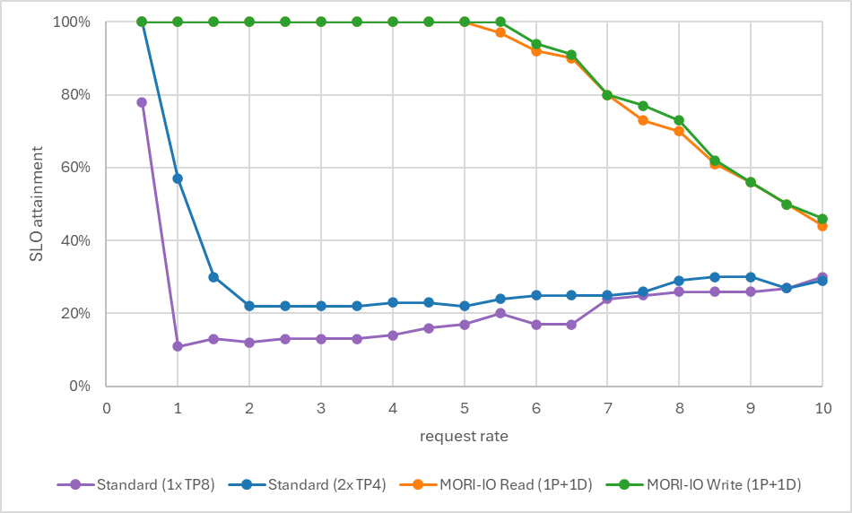
图 4 展示了从 0.5 到 10 req/s 的 SLO 达成率:
- Standard(1× TP8): 从低请求率开始就出现 ITL 违规,在所有测试请求率下占主导地位。在 rate=8 时达成 26/100。
- Standard(2× TP4): 急剧下降——从 rate=0.5 的 100% 到 rate=1 的约 60%,到 rate=2 时崩塌到约 25% 并趋于平缓。ITL 违规在早期就饱和了。
- MORI-IO Read(1P+1D): 在 rate~5 之前保持 100% 达成率,然后逐渐下降到 rate=10 时的约 44%,主要因 TTFT 开始超标。
- MORI-IO Write(1P+1D): 在 rate~5.5 之前保持 100% 达成率,然后逐渐下降到 rate=10 时的约 46%,主要因 TTFT 开始超标。
理解权衡
为什么 ITL 会改善
在标准部署中,prefill 和 decode 共享同一个 vLLM 引擎,在同一个 batch 内竞争调度。单个 prefill——在一次前向传播中处理所有输入 token——所需时间远长于一个 decode 步骤。同一 batch 中的每个 decode 请求都必须等待该 prefill 完成才能生成下一个 token,这直接拉长了 ITL。
有了分离,你的 decode 引擎只运行纯粹 decode 的 batch。没有计算密集的 prefill 任务打断步骤节奏,因此无论系统有多少新请求进入,ITL 都变得稳定和可预测。这一优势在 read 模式和 write 模式下完全相同——两种情况下 decode 引擎都与 prefill 隔离。
为什么 TTFT 会变差
另一方面:分离增加了首 token 路径的开销。在标准部署中:
TTFT = queue + prefill_forward_pass + sample_T1 + detokenize + SSE_encode + network在 read 模式下,插入了两个额外步骤(图 5):
TTFT = queue(prefill) + prefill_forward_pass
     + [proxy serialization: await prefill, dispatch to decode]  <- 开销 1
     + RDMA transfer (WAITING_FOR_REMOTE_KVS)                   <- 开销 2
     + queue(decode) + sample_T1 + detokenize + SSE_encode + network
在 write 模式下(图 6):
TTFT ≈ max(
           queue(prefill) + prefill_forward_pass + RDMA_write_time,
           queue(decode)
       ) + sample_T1 + detokenize + SSE_encode + network
Write 模式消除了开销 1。由于 proxy 并发分派到两个实例,decode 队列等待和 prefill 计算重叠。剩余的成本——RDMA 传输本身——在结构上与 read 模式中的 RDMA 读取是等价的。
开销 1:Proxy 序列化(仅 Read 模式)
在 read 模式下,proxy 在分派给 decode 之前等待完整的 prefill 响应。这导致整个 prefill 计算时间加上一次 proxy 往返被计入客户端可见的 TTFT。在 write 模式下,这一阻塞被跳过——decode 请求在 prefill 完成前已经在飞行中。
# examples/online_serving/disaggregated_serving/moriio_toy_proxy_server.py

if TRANSFER_TYPE == "READ":
    # 在 read 模式下,prefill 和 decode 串行执行
    prefill_response = await send_prefill_task
    req_data["kv_transfer_params"]["remote_engine_id"] = prefill_response[
        "kv_transfer_params"
    ]["remote_engine_id"]
    req_data["kv_transfer_params"]["remote_block_ids"] = prefill_response[
        "kv_transfer_params"
    ]["remote_block_ids"]
开销 2:RDMA 传输等待
一旦 decode 实例收到请求,它进入 WAITING_FOR_REMOTE_KVS 状态。调度器每一步跳过该请求,直到 RDMA 传输完成,然后立即将其移到 ready 队列进行调度。
# vllm/v1/request.py

WAITING_FOR_REMOTE_KVS = enum.auto()

# vllm/v1/core/sched/scheduler.py
# KVTransfer: 如果仍在等待远端 kvs,跳过该请求

if request.status == RequestStatus.WAITING_FOR_REMOTE_KVS:
    is_ready = self._update_waiting_for_remote_kv(request)
    if is_ready:
        request.status = RequestStatus.WAITING
    else:
        logger.debug("%s is still in WAITING_FOR_REMOTE_KVS state.",
                     request.request_id)
        self.waiting.pop_request()
        skipped_waiting_requests.prepend_request(request)
        continue
在 read 模式下,这个等待在 prefill 已经完成后才开始。在 write 模式下,这个等待在 decode 请求到达时立即开始——与另一个实例上正在进行的 prefill 计算重叠。
底线: 分离给你稳定、可预测的 ITL,代价是第一 token 的等待时间更长。具体长多少取决于模式。在 read 模式下,TTFT 至少增加一整个 prefill 前向传播(proxy 序列化)加上 RDMA 传输时间。在 write 模式下,proxy 序列化被消除——TTFT 仅增加 RDMA 传输时间,该时间与 prefill 计算重叠,因此净惩罚更小。无论如何,ITL 的收益是相同的。
何时应该使用?
表 4 总结了不同情况下应优先选择的部署方案。
| 你的情况 | 建议 |
|---|---|
| 生产负载下 ITL p99 超出 SLO | 分离——这是主要使用场景 |
| TTFT 是你的硬约束(如聊天机器人 UX) | 标准部署可能更优 |
| 高并发 + 长 prompt | 分离——prefill 干扰在此最严重 |
| 低请求率 + 短 prompt | 标准部署足够 |
如何设置
现在你已经看到了结果,以下是部署方法。你需要配置三个组件:prefill 实例、decode 实例和 proxy 服务器。完整的 vLLM 分离式 prefill 文档见 [2]。
Prefill 实例
Prefill 实例充当 KV 生产者(kv_role: kv_producer)。它处理输入 prompt,计算 KV cache,并通过 RDMA 使其对 decode 实例可用。
vllm serve <model> \
  ...
  --gpu_memory_utilization 0.9 \
  --kv-transfer-config '{
    "kv_connector": "MoRIIOConnector",
    "kv_role": "kv_producer",
    "kv_connector_extra_config": {
      "proxy_ip": "127.0.0.1",
      "proxy_ping_port": "36367",
      "http_port": "20005",
      "handshake_port": "6301",
      "notify_port": "6105"
    }
  }'
启动时,实例通过 ZMQ 向 proxy 注册自己,发送其角色、HTTP 地址、握手和通知端口以及并行配置。它会持续发送周期性注册消息,以便 proxy 检测不可用状态。
Decode 实例
Decode 实例充当 KV 消费者(kv_role: kv_consumer)。它在 prefill 完成后从 proxy 接收请求,然后通过 RDMA 拉取 KV cache。
vllm serve <model> \
  ...
  --gpu_memory_utilization 0.9 \
  --kv-transfer-config '{
    "kv_connector": "MoRIIOConnector",
    "kv_role": "kv_consumer",
    "kv_connector_extra_config": {
      "proxy_ip": "127.0.0.1",
      "proxy_ping_port": "36367",
      "http_port": "40005",
      "handshake_port": "7301",
      "notify_port": "7501"
    }
  }'
Proxy 服务器
Proxy 是一个轻量级 HTTP 服务器,编排两阶段流程。它通过 ZMQ 在 proxy_ping_port 上监听实例注册,并使用轮询(round-robin)调度路由每个请求。
python examples/online_serving/disaggregated_serving/moriio_toy_proxy_server.py在 READ 模式下,proxy 等待 prefill 实例完成,从响应中提取 remote_block_ids,并将其传递给 decode 实例,使其确切知道要拉取哪些 KV block。
端口参考
每个实例使用多个端口用于不同的通信通道,汇总于表 5。每个 rank 的偏移量在 MoRIIOConfig 中应用(参见 moriio_common.py):
| 端口 | 用途 |
|---|---|
proxy_ping_port | ZMQ 端点,每个实例通过它向 proxy 注册 |
http_port | vLLM HTTP 服务器端口;proxy 在此转发推理请求 |
handshake_port | 一次性元数据交换:消费者获取生产者的 KV cache 布局 |
notify_port | 每请求同步:prefill 向 decode 发出 KV block 就绪信号 |
实验细节
搭建环境
可通过提供的 Dockerfile 复现环境——Dockerfile.rocm_base(使用 MORI commit 2d02c6a9,来自 ROCm/mori)和 Dockerfile.rocm(使用 vLLM main 分支,来自 vllm-project/vllm)。
硬件:
- GPU:8× AMD Instinct MI300X GPU(gfx942)
- CPU:2× AMD EPYC 9654 96-Core Processor
软件栈:
- ROCm Driver:6.10.5(AMDGPU)
- Container:rocm/vllm-dev(ROCm 7.0.51831-a3e329ad8)
- vLLM:0.16.0rc1.dev1+gc46b0cd0a(git sha: c46b0cd0a)
- PyTorch:2.9.1+git8907517(ROCm 7.0.51831-a3e329ad8)
- MORI 库:commit c365eaed
基准测试配置:
- 模型:Qwen/Qwen3-235B-A22B-FP8
- 输入序列长度:2000 tokens
- 输出序列长度:1000 tokens
- 数据集:random
- 工作负载:100 个总请求
- 请求率:0.5 到 10(步长 0.5)
基线配置
本文中比较的四种配置如表 6 所述:
| 配置 | 描述 |
|---|---|
| Standard(1× TP8) | 单个 vLLM 实例使用所有 8 块 MI300X GPU(TP=8),启用 expert parallelism。在一个引擎上处理混合的 prefill 和 decode 工作负载。 |
| Standard(2× TP4) | 两个相同的 vLLM 实例,各使用 4 块 MI300X GPU(TP=4),启用 expert parallelism。轮询 proxy 均匀分配请求。两个实例均处理混合的 prefill 和 decode 工作负载。 |
| MORI-IO Read(1P+1D) | 一个 prefill 实例(GPU 0–3)和一个 decode 实例(GPU 4–7),各 TP=4,启用 expert parallelism。两个实例上均设置 VLLM_MORIIO_CONNECTOR_READ_MODE=1。Proxy 串行分派:等待 prefill 返回 remote_block_ids,然后转发给 decode。Decode 通过 RDMA 拉取 KV cache。禁用 prefix caching。 |
| MORI-IO Write(1P+1D) | 一个 prefill 实例(GPU 0–3)和一个 decode 实例(GPU 4–7),各 TP=4,启用 expert parallelism。通过 MORI-IO write 模式传输 KV cache。有状态 proxy 编排两阶段路由。禁用 prefix caching(MORI-IO connector 要求)。 |
为什么要选这个基线? Standard(2× TP4)和分离配置都使用相同的 GPU 总数(8 块 MI300X)分为两个 4-GPU 组,确保公平的逐项对比。唯一的区别在于每组运行的是混合 prefill+decode 工作负载(标准)还是专用的 prefill 或 decode 工作负载(分离)。Standard(1× TP8)作为额外参考点,在一个引擎中使用全部 8 块 GPU。
通用性说明: 这些结果使用 Mixture-of-Experts(MoE)模型(Qwen3-235B-A22B-FP8)。Prefill/decode 干扰模式是 transformer 推理的基础性问题,同样适用于密集模型。MoE 模型往往会放大这一效应,因为专家路由增加了每步计算的可变性,使 ITL 抖动更加明显。
结论与未来方向
本文证明了 PD 分离不仅仅是数据中心级技术——它在一台 8-GPU 节点上也能带来可测量的收益。通过将 GPU 专用于每个阶段,并使用 MORI-IO 进行高效的基于 RDMA 的 KV cache 传输,我们实现了 2.5 倍更高的 goodput,并消除了困扰混杂部署的 ITL 违规问题。
下一步计划
- 多节点部署: 生产中,prefill 和 decode 实例可跨多个节点——MORI-IO 已通过网络架构使用 RDMA,因此同一个 connector 无需代码修改即可跨主机工作。
- 按阶段调优: 有了专用实例,prefill 实例可以配置为高计算吞吐(更大的 token budget、chunked prefill),而 decode 实例则针对低延迟调优(更小的 batch size、更严格的调度)。这种独立旋钮调节在混杂部署中是不可能的。
附录:可复现配置
要复现这些结果,预构建的 nightly 镜像可在 rocm/vllm-dev 获取,或从 vLLM 仓库中的 Dockerfile.rocm_base 和 Dockerfile.rocm 源码构建(MORI commit 2d02c6a9,vLLM commit c46b0cd0a)。
所有基准测试的完整 vLLM 命令行配置如下。每个命令包括环境变量、并行度标志以及在 AMD Instinct MI300X GPU 上部署 Qwen3-235B-A22B-FP8 的参数。
标准部署
# 实例 1(GPU 0-3)
CUDA_VISIBLE_DEVICES=0,1,2,3 VLLM_ROCM_USE_AITER=1 vllm serve Qwen/Qwen3-235B-A22B-FP8 \
  -tp 4 \
  --enable-expert-parallel \
  --max-model-len 16384 \
  --max-num-batched-tokens 8192 \
  --distributed-executor-backend mp \
  --no-enable-prefix-caching \
  --port 8100

# 实例 2(GPU 4-7)
CUDA_VISIBLE_DEVICES=4,5,6,7 VLLM_ROCM_USE_AITER=1 vllm serve Qwen/Qwen3-235B-A22B-FP8 \
  -tp 4 \
  --enable-expert-parallel \
  --max-model-len 16384 \
  --max-num-batched-tokens 8192 \
  --distributed-executor-backend mp \
  --no-enable-prefix-caching \
  --port 8200

# Proxy
cd <path_to>/vllm
python benchmarks/disagg_benchmarks/round_robin_proxy.py
分离式部署
# Prefill 实例(GPU 0-3)
export VLLM_MORIIO_CONNECTOR_READ_MODE=1    # 取消设置以启用 write 模式
export VLLM_ROCM_USE_AITER=1
export CUDA_VISIBLE_DEVICES=0,1,2,3
export HIP_VISIBLE_DEVICES=0,1,2,3
export MORI_DISABLE_AUTO_XGMI=1
export MORI_IO_ENABLE_NOTIFICATION=0

vllm serve Qwen/Qwen3-235B-A22B-FP8 \
  -tp 4 \
  --enable-expert-parallel \
  --port 20005 \
  --max-num-batched-tokens 4096 \
  --distributed-executor-backend mp \
  --gpu_memory_utilization 0.9 \
  --max-model-len 16384 \
  --max_num_seqs 64 \
  --no-enable-prefix-caching \
  --kv-transfer-config '{
    "kv_connector": "MoRIIOConnector",
    "kv_role": "kv_producer",
    "kv_connector_extra_config": {
      "proxy_ip": "127.0.0.1",
      "proxy_ping_port": "36367",
      "http_port": "20005",
      "handshake_port": "6301",
      "notify_port": "6105"
    }
  }'

# Decode 实例(GPU 4-7)
export VLLM_MORIIO_CONNECTOR_READ_MODE=1    # 取消设置以启用 write 模式
export VLLM_ROCM_USE_AITER=1
export CUDA_VISIBLE_DEVICES=4,5,6,7
export HIP_VISIBLE_DEVICES=4,5,6,7
export MORI_DISABLE_AUTO_XGMI=1
export MORI_IO_ENABLE_NOTIFICATION=0

vllm serve Qwen/Qwen3-235B-A22B-FP8 \
  -tp 4 \
  --enable-expert-parallel \
  --port 40005 \
  --no-enable-prefix-caching \
  --max-num-batched-tokens 4096 \
  --distributed-executor-backend mp \
  --gpu_memory_utilization 0.9 \
  --max-model-len 16384 \
  --max_num_seqs 64 \
  --kv-transfer-config '{
    "kv_connector": "MoRIIOConnector",
    "kv_role": "kv_consumer",
    "kv_connector_extra_config": {
      "proxy_ip": "127.0.0.1",
      "http_port": "40005",
      "proxy_ping_port": "36367",
      "handshake_port": "7301",
      "notify_port": "7501"
    }
  }'

# Proxy
cd <path_to>/vllm
python examples/online_serving/disaggregated_serving/moriio_toy_proxy_server.py
致谢
我们感谢许多为本次合作贡献力量的优秀人才:
AMD: Hongxia Yang, Gilbert Lei, Mingzhi Liu, Niko Ma, Tian Di, Randall Smith, Feiyue Zhai, Peng Sun,以及 MORI 团队。
Embedded LLM: Pin Siang Tan, Jun Kang Chow, Ye Hur Cheong, Vensen Mu, Jeff Aw, Tun Jian Tan,以及 Embedded LLM 团队。
参考文献
- AMD and Embedded LLM, “The vLLM MoE Playbook: A Practical Guide to TP, DP, PP and Expert Parallelism” https://rocm.blogs.amd.com/software-tools-optimization/vllm-moe-guide/README.html
- vLLM Disaggregated Prefill Documentation https://docs.vllm.ai/en/latest/features/disagg_prefill/
- DistServe: Maximizing Goodput in LLM Serving https://haoailab.com/blogs/distserve/
- MORI-IO Connector PR #29304 https://github.com/vllm-project/vllm/pull/29304
- MORI (Modular RDMA Interface) https://github.com/ROCm/mori
免责声明
测试时间为 2026 年 3 月 12 日,在 AMD Instinct MI300X 平台上测量推理 goodput。
硬件配置
MI300X:AMD EPYC 9654 96-Core Processor 服务器,8× AMD Instinct MI300X(192GB, 750W)GPU,NPS1(每 socket 1 NUMA),2.2TiB(24 DIMMs, 4800 MT/s 内存, 96 GiB/DIMM)
软件配置
Ubuntu 22.04 LTS,Linux kernel 5.15.0-153-generic,ROCm Driver 6.10.5(AMDGPU),ROCm 7.0.51831-a3e329ad8,PyTorch 2.9.1+git8907517,vLLM 0.16.0rc1.dev1+gc46b0cd0a,MORI 库 commit c365eaed
服务器制造商可能配置各异,导致不同结果。性能可能因配置、软件、vLLM 版本以及使用最新驱动和优化而有所不同。
原文:Next-Level Inference: Why Your Single-Node vLLM Setup Needs Prefill-Decode Disaggregation — vLLM Blog, April 7, 2026